Counting to meaning

Last time, I've talked about distributional semantics in rather vague terms, or what we scientists call "theory". Let's try to get a bit more precise this time around. We'll be looking at a simple model based on occurrence counts. The main purpose of this post is to sketch a general idea of what distributional semantics models look like.

To recap, distributional semantics is the theory of meaning according to which word distribution correlates with word meaning. The contexts in which a word is likely to occur are constrained by what that word means. Models of distributional semantics are concrete implementations of this theory. A distributional semantics model (or DSM for the lazy writer) will give a meaning description for every possible word—or at least attempt to. This is a rather broad definition, and in fairness it could be applied to quite a number of very different things; but we'll get to that in future posts.

One thing to point out is that any computation that gives the conditional probability of a word given the sentence it occurs in can be construed as a DSM. If I have some metric that shows that the word "rabbits" is more likely than the word "clergymen" in the sentence "My pet ______ are adorable", then I have a metric that characterize word distribution; and if I assume that the distributional hypothesis is correct, I can infer that this metric also characterizes meaning.

Here, "conditional probability" is to be understood in the strict mathematical sense. When we talk of the probability of some event, we just mean a score between 0 and 1 of how likely that event is. As an added rule, we want mutually exclusive events to have scores that sum to 1. So, suppose we flip a coin: the coin must either end up heads up or tails up; if my coin is fair, the probability of it landing heads up should be the same as it landing tails up. Hence the probability of a fair coin landing heads up would be 0.5.

Conditional probabilities, now, are probability scores that we have updated: something has happened; we know more stuff now, and we can say that all outcomes are no longer exactly as likely as they were previously.

As a simple example, imagine I am randomly picking colored balls from a vase, which contains five red balls and five blue balls. At the beginning, it is equally likely that I pick a red or a blue ball: each event has a probability of 5/10. Say I've picked a red ball: there are now four red balls and five blue balls in my vase. Given that I picked a red ball at the first round, the probability that I pick a blue one is no longer 0.5, but 5/9; likewise, the probability that I pick a red ball is now no longer 0.5 but 4/9.

This is a rather simple approach: we can just count stuff, be it colored balls or coin faces, and from that we should be able to characterize how likely are all outcome events.

Going back to our DSMs, we can use this notion of conditional probability to characterize word distributions. What is the probability that the word "rabbits" occur in a sentence, given that the word "burrows" also occurs in it? To answer that, I can just grab a large corpus of text, and count the number of sentences that contain the word "burrows", and compute the proportion of those that also contain the word "rabbits". I can do the same using "clergymen" instead of "rabbits". I can also characterize the distribution of these two words using some other observation: for instance, how the occurrence of the word "cathedral" constrains the distribution of "rabbits" and "clergymen".

Intuitively, you expect "rabbits" to occur more frequently with "burrows" than with "cathedral", and you expect the opposite for "clergymen". Let's look at real data and see whether this holds water. Grabbing any old corpus of English I have sitting on my laptop, out of 1847 sentences containing "carrots", exactly 18 contain the word "rabbits" and 0 contain the word "clergymen". Out of the 15088 sentences containing "cathedral", 0 contain the word "rabbits", and 5 contain the word "clergymen".

What is neat about this sort of approach is that we can extend it to any word. Don't trust me? Well, let's walk through one more: "dragons" occurs once with "burrows", and 4 times with "cathedral". In fact, we can even plot these observations in a 2-dimensional plane: let's have the x-axis be the number of times we observe a word in the same sentence as "burrows", and y-axis the number of times we observe it with "cathedral". That would give us something like the vectors in the following picture:

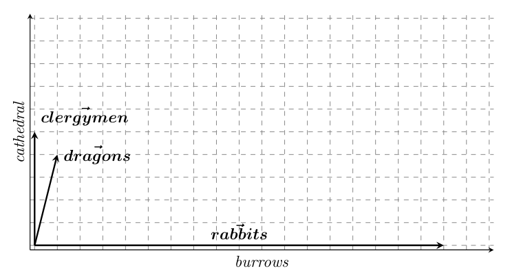
And let there be word vectors! We get representations of words, computed from their distributions, that correspond to points in some abstract space of (probabilistic) observations. That's where the "word vectors" I study come from—although to be fair, what I have presented here is a very simplified approach.

So... Are dragons more like clergymen that rabbits? At least, our 2D vectors in the image above suggest that it is the case. And you have to admit that, yes, it's more likely you'll hear about some holy bishop driving out a terrible dragon than Bugs Bunny doing so. In fact, this hints at a core characteristic of DSMs: they are usage-based and data-driven. What you get out of your representations depends on what data you've put into the model.

Another point to stress is that dragons are more like clergymen than rabbits only if we limit ourselves to the two tests we came up with. It's important to consider that we can extend our methodology to any and all words in the vocabulary. But that would lead to impractical high-dimensional vectors. How many dimensions, you ask? There are 5,008,462 different word types in the corpus we've used to compute our representations. We'd need 5,008,460 more dimensions if we were to take into account all the vocabulary data we have.

I'll stop here for today. Hopefully it wasn't too hard to follow. Next time, we'll look at a more recent (and therefore more complex) DSM architecture. In the meantime, here's some unrelated piece of entertainment for you.