Gradient Descent into madness

I did my best to convince you to stop reading. I discussed dry, nitpicky theoretical arguments to distinguish between two fields that are essentially the same. I made lame duck jokes. I talked about old, dusty, mouldy dictionaries. And yet you chose to remain here. Whatever comes next is on you.

Today's topic is calculus. Matrix calculus.

Disclaimer first: I am not going to discuss the gruesome math equations in much details. My aim in this post is to give you, the reader, an idea of how neural networks function and "learn" stuff.

Neural networks are a major component of my everyday work. If you grab me at any point of the day, chances are I am doing one of the following:

1. Read scientific papers
2. Write scientific papers
3. Drink coffee, and chat with colleagues
4. Clean up data
5. Run experiments, generally using neural networks

The first thing you need to know about neural networks is that they are models. We try to represent some phenomenon by means of a mathematical setup that hopefully will generalize to unseen data.

Let's take a concrete example: suppose I am a hardy biologist. I am interested in the correlation between duck size and duck violence: I have observed that bigger ducks tend to be more dangerous. As I am a scientist, I've plotted the number of violent acts against the size of the mallards:

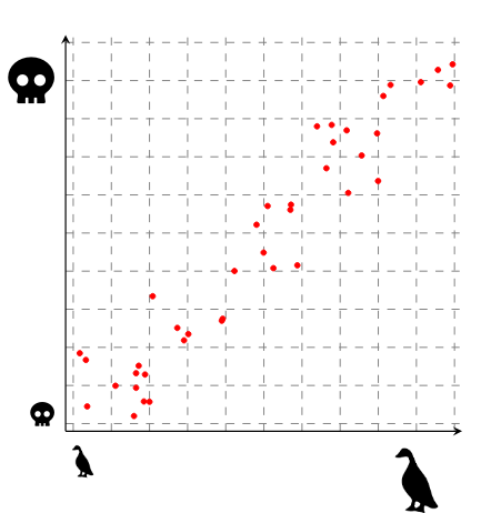
Instead of handling all these data points separately, we would like a handy formula that gives the expected violence of a duck given its size. A formula that works, i.e., generalizes well to unseen data, is a way of making science, because science is all about generalizing.

Here, my plot suggest that there is indeed a correlation between duck size and duck violence. In fact, it looks linear: I could draw a straight line through my data points that fit nicely. As a reminder, the equation for a straight line is y = mx + b. Here, m would be the slope (i.e., how steep the line is: 0 is a flat line and infinity is a vertical line) and b is the bias (i.e., where our line crosses the y-axis). If I try to find this line, I can draw something like that:

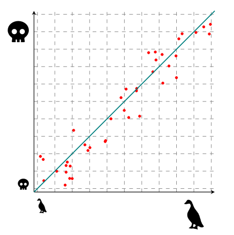
If this line has a slope m and a bias b, I can now use it to do science: for any duck I meet, I can measure its size, multiply it by m and add b, and that will give me how violent that duck is. But here's the hard question: how do I get m and b?

In machine learning jargon, m and b are the parameters of our model. We could have more than two; in fact, many neural networks have thousands of parameters, if not millions or more. The equations we fit are also more complex than the simple line I described here. Lastly, we rarely start from a single input: here we have only the size, but a more realistic models might take into account the age, the color, the habitat, etc.

In any event, we are trying to fit parameters to our data. Let's go back to our duck example. First things first: how do we get started? Well, to begin with, we can just try anything: we'll pick random values for m and b, and see how it goes.

But wait—how do we "see how it goes"? Here's where another important concept comes in: we need some way of quantifying how wrong our model currently is. In machine learning parlance, that's what we'd call a criterion or a loss. With this loss function L, we can compare the prediction of the model ŷ to the target value y. In the specific case of our duckline, we are interested in predicting numbers, so we can use something rather simple: L(ŷ, y) = (y - ŷ)², viz. the squared difference between the prediction and the target. That function has some interesting properties: (1) it is equal to 0 if and only if our prediction matches the target perfectly, (2) the more we undershoot or overshoot the target, the bigger the loss function will be. Hence, I can say it measures how bad the model currently is.

Let's plot it and have a look:

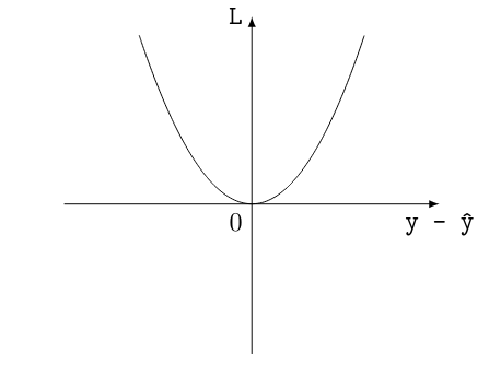
If the difference between ŷ and y is 0, I get 0. Anything else will blow up to higher and higher values for my loss function. To sum up: we made a first random guess for our parameters, and then we quantified how bad that guess was. Now what?

That's where the calculus comes in. Let's compare two scenarios: one where the model was very wrong, and one where it was less wrong. We can mark the error of the model in each scenario, and then compute how much the loss is increasing at this point. This we do by computing the derivative (i.e., the tangent at that point): as a reminder, the derivative describes how much a function increases at any point. Here's a visual aid:

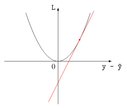
A very wrong guess

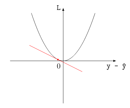
A less wrong guess

As we can see, the less wrong guess will correspond to a flatter tangent. This tells us that we are more likely to be near the absolute minimum loss: that is to say, we're almost at 0. The other important bit to take notice of is that the trend of the tangent also tells us something: if the slope is going downwards, I'm overshooting the target value, whereas if it is going upward, I'm undershooting it.

To clarify: by computing the derivative, we can get two very useful clues: how far away am I from the minimum (by looking at how flat the tangent is), and whether I should make smaller or bigger guesses (by looking at the trend of the tangent). These two clues tell us how we should correct our first random guess: the first tells us the magnitude of the change we should perform, the second tells us the sign.

The last thing we need now is how to translate these clues into concrete updates to our parameters. That is to say: given these two clues, how do I tweak m and b? The answer is that we use partial derivatives: instead of computing the full derivative as we did above, we compute the derivative of the loss with respect to each parameter, and other parameters and inputs are treated as constant values.

In other words: we look at how we should change a parameter to get a less wrong answer, if the only thing we could change was this single parameter. Hence the clues we get from the partial derivative apply specifically to this one parameter, and we can use the flatness to determine how big of a change we should do, and the trend to tell us whether we should make that change towards more negative values or towards more positive values.

This gives us a way to update our initial random guess. Keep in mind that this is just an update: in practice, we'll have to go through the whole process of computing the loss and the partial derivatives a great number of times before the model finally finds the 0, or, as we say, converges to a solution. This mechanism as a whole is what we call gradient descent.

This duck example was fairly silly. One point that I have completely ignored is that we don't work with number in NLP: instead, we work with words, or parts of speech, or syntactic trees, etc. This means that in the general case, what we predict is a probability distribution over all possible words, and the loss function is generally one that quantifies how two distributions differ. More on that in future posts! You've probably suffered enough math for today.

The other thing that I really should point out as early as possible is that real machine learning applications have real consequences. The main issue is that neural networks will use any random correlation in your dataset to converge to a solution. If you want to predict where crime is likely to occur using police reports, you're in fact going to predict where overpolicing occurs. If you want to build an application that unlocks a phone by scanning the user's face, but your dataset is full of white dudes between 20 and 35, then your application will not work with any other demographic. I'll try talk about this as well.

See you next time.